Introduction

High-Speed Rail (HSR) investments represent some of the most capital-intensive and transformative infrastructure projects that a nation can undertake. In the context of Australia, the proposed East Coast HSR corridor connecting Newcastle, Sydney, Canberra, and Melbourne represents a nation-shaping initiative designed to address long-term settlement patterns, metropolitan congestion, and regional productivity differentials (Henn et al., 2012). Traditionally, such transport megaprojects have been appraised using standard Cost-Benefit Analysis (CBA) frameworks rooted in partial equilibrium (PE) economic theory (Department for Transport, 2005). However, these PE frameworks are conceptually constrained, as they assume that the transport sector exists in isolation from the broader economy and that prices equal marginal costs in all other markets (Hörcher & Graham, 2026). Under these assumptions, the wider economic impacts (WEIs) of transport investments, such as agglomeration economies, labour supply responses, and property capitalisation, are either omitted entirely or added ex-post using ad-hoc, aggregate elasticities that risk double-counting benefits (Wegener, 2011; Graham & Gibbons, 2019).

To capture the spatial and temporal feedback loops triggered by massive connectivity enhancements, urban planners and transport economists have turned to Land-Use Transport Interaction (LUTI) models and, more recently, Quantitative Spatial Models (QSMs) in spatial general equilibrium (Redding & Rossi-Hansberg, 2017). Yet, both paradigms suffer from distinct and significant limitations. Traditional LUTI models, while behaviorally rich and highly disaggregated, lack a single, unified microeconomic welfare utility function (Eliasson & Fosgerau, 2019). Consequently, they cannot produce a mathematically consistent, closed-form measure of aggregate welfare changes, making them unsuitable for formal economic appraisal. Conversely, state-of-the-art QSMs are theoretically consistent and mathematically elegant, but they achieve tractability by making highly restrictive transport assumptions, such as static routing, exogenous transport networks, “iceberg” travel costs, and the complete exclusion of non-commuting trips (Anas & Liu, 2007; Proost & Thisse, 2019).

This paper resolves this methodological divide by presenting a new LUTI model approach: a two-stage calibration-simulation workflow that reconciles the rigorous welfare-theoretic foundations of Spatial General Equilibrium (SGE) with the high-resolution behavioural realism of agent-based microsimulation (MATSim and UrbanSim). The temporal causal chain of our framework explicitly distinguishes between short-run travel responses (0 to 2 years), medium-run firm relocations (2 to 10 years), and long-run household migration and real estate developments (10 or more years) (Acheampong & Silva, 2015). By sequencing the execution of our model components along this temporal causal chain, we establish a mathematically consistent, market-clearing equilibrium across transport, labour, and property markets.

Our contribution is threefold:

1. We formalise a two-stage calibration-simulation protocol that overcomes the “invertibility-microsimulation” bottleneck, enabling researchers to recover unobserved locational fundamentals algebraically and simulate agent-based behaviors within a general equilibrium framework.

2. We derive a unified, non-overlapping general equilibrium welfare decomposition based on the latest advances in spatial economics (Donald et al., 2025; Hörcher & Graham, 2026), allowing direct benchmarking against traditional CBA components.

3. We conceptually apply this hybrid architecture to the Newcastle-to-Melbourne HSR corridor, showing how different spatial outcomes, including metropolitan agglomeration, regional function-borrowing, and commuter-town capitalisation, emerge under different policy and land-use scenarios.

The paper is structured as follows. Section 2 reviews and critiques the prevailing transport appraisal paradigms. Section 3 defines the microeconomic foundations of our household utility maximisation model. Section 4 presents the general equilibrium market-clearing conditions. Section 5 details the agent-based coupling protocol between MATSim and UrbanSim. Section 6 applies the methodology conceptually to the East Coast HSR corridor. Section 7 outlines the welfare economic decomposition. Section 8 discusses the model’s limitations and future research agenda, and Section 9 concludes.

Literature review and paradigm critique

To contextualise the proposed hybrid architecture, it is necessary to examine the theoretical and empirical deficiencies of the three leading transport-land use appraisal methodologies: Partial Equilibrium (PE), Land-Use Transport Interaction (LUTI), and Quantitative Spatial Models (QSM).

The partial equilibrium (PE) tradition and standard CBA

Standard transport appraisal frameworks are almost exclusively built upon partial equilibrium economics (Dupuit, 1844; Marshall, 1920). These models focus on the transport market in isolation, measuring changes in consumer surplus via travel time savings (TTS) and vehicle operating cost reductions (Department for Transport, 2005). The fundamental assumption of PE is that price equals marginal cost in all secondary markets, meaning that any transport-induced changes in labour supply, firm productivity, or property values are merely reallocations of the direct transport user benefits (Venables, 2007). Under perfect competition, these secondary changes represent zero net welfare additions.

However, real-world economies are characterised by persistent market failures, including imperfect competition, monopolistic pricing, agglomeration externalities, and labour market distortions (SACTRA, 1999). When these imperfections exist, a transport improvement triggers wider economic impacts (WEIs) that are not captured by direct user benefits (Graham & Gibbons, 2019). While standard guidelines allow for the ex-post addition of WEIs (such as agglomeration productivity gains), these additions are calculated using aggregate, static indicators (such as effective density) that fail to capture the dynamic re-sorting of households and firms (Joint Transport Research Centre, 2008). Furthermore, PE models cannot account for the capitalisation of transport benefits into land values and the subsequent feedback on housing supply, which can severely distort the final benefit-cost ratio (Beria et al., 2012).

Land-use transport interaction (LUTI) models

LUTI models were developed to endogenise the relationship between transport and the spatial distribution of activities (Lowry, 1964; Hunt & Simmonds, 1993). Modern aggregate LUTI models (such as MEPLAN or TRANUS) simulate how changes in transport costs alter accessibility, which in turn drives household residential choices and firm location decisions (Echénique et al., 1990; Wegener, 2011). While these models are highly disaggregated and capable of predicting spatial reallocations, they have been widely criticised by economists for their lack of microeconomic rigor (Eliasson & Fosgerau, 2019).

The primary limitation of traditional LUTI models is that they are not micro-founded under a single, unified welfare utility function. Instead, they typically couple a gravity-based or logit transport model with an independent, heuristic land-allocation model. Because the household’s residential choice utility is not mathematically consistent with the traveller’s mode and route choice utility, it is impossible to derive a closed-form, theoretically consistent measure of aggregate welfare (Wegener, 2004). This theoretical inconsistency leads to the “double-counting” dilemma, where planners struggle to separate direct transport benefits from land value capture and productivity gains, leading to arbitrary and unreliable appraisal outcomes (Tudela et al., 2006).

Quantitative spatial models (QSM) and spatial general equilibrium (SGE)

Since the mid-2010s, Quantitative Spatial Models (QSMs) have revolutionised spatial economics by combining general equilibrium consistency with empirical tractability (Ahlfeldt et al., 2015; Redding & Rossi-Hansberg, 2017). QSMs feature a powerful mathematical property known as model inversion, which allows researchers to work backward from observed census data (such as population counts, wages, and property prices) to deterministically recover unobserved “locational fundamentals,” such as residential amenities, workplace amenities, and baseline firm productivity, as structural residuals (Monte et al., 2018).

Despite their theoretical elegance, current QSMs make highly unrealistic transport assumptions to preserve analytical tractability:

1. Iceberg Travel Costs: Most QSMs model transport costs as an ad-valorem utility tax (iceberg cost), assuming that a fraction of the traveller’s utility melts away during travel (Donaldson, 2018). This formulation conflates travel times with monetary fares, preventing the explicit modelling of travel budgets and fare structures.

2. Static Routing and Absence of Congestion: QSMs typically rely on simple, exogenous network matrices, completely ignoring route choice and endogenous link-level congestion (Anas & Liu, 2007).

3. Exclusion of Non-Commuting Trips: To maintain mathematical tractability, QSMs restrict their focus to simple commuting trips, failing to capture the complex, multi-purpose trip chains (such as shopping, leisure, and business travel) that dominate modern urban transport (Miyauchi et al., 2025).

Our proposed new LUTI model approach directly addresses these gaps by coupling an invertible SGE model with agent-based transport and land-use microsimulation engines (MATSim and UrbanSim).

Mathematical foundations of the household problem

Our framework establishes a rigorous microeconomic foundation for households, building upon and extending the transport-oriented spatial model of Hörcher and Graham (2026). Let the spatial economy consist of n discrete geographic locations indexed by i (representing residence) and j (representing workplace), connected by a multimodal transport network.

Household preferences and nested cobb-douglas utility

A representative household choosing to reside in location i and commute to work in location j derives utility from leisure time, the consumption of non-tradable goods, and residential floorspace. The utility function is specified as:

U_ij = (L_ij^1 − γ)^1 − γ(K_ij^γ)^γz_ij

where L_ij is individual leisure time, K_ij is a composite consumption and housing subutility, γ ∈ (0, 1) is a structural preference parameter, and z_ij is an idiosyncratic taste shock associated with the combination of residence i and workplace j. The subutility K_ij is defined as:

K_ij = (C_ij^β)^β(H_ij^{R(1 − β)})^1 − β

where C_ij represents the consumption of a tradable numeraire good (whose price is normalised to 1 across all zones), H_ij^R is the consumption of residential floorspace at residence i, and β ∈ (0, 1) dictates the household budget share allocated to tradable goods versus housing.

Separate monetary and temporal constraints

Unlike conventional QSMs that use simple income deductions, households in our model face separate, binding temporal and pecuniary constraints. The monetary budget constraint is:

x_ij(w_j − τ_ij) = C_ij + q_iH_ij^R

where w_j is the wage rate paid at workplace j, τ_ij is the round-trip monetary travel fare between i and j, q_i is the residential floorspace price in residence i, and x_ij is the continuous individual labour supply (representing the number of workdays supplied by the individual).

The temporal budget constraint for the representative day is:

|(L) = L_ij + x_ij(T + t_ij)

where |(L) is the daily active time endowment (typically set to 24 hours), T is the fixed length of a standard workday (typically 8 hours), and t_ij is the round-trip travel time between residence i and workplace j.

Optimisation and derivation of the lagrange multipliers

To solve the household’s utility maximisation problem, we define the Lagrangian function:

Λ = U_ij − κ_ij[C_ij + q_iH_ij^R − x_ij(w_j − τ_ij)] − μ_ij[L_ij + x_ij(T + t_ij) − |(L)]

where κ_ij and μ_ij are the Lagrange multipliers representing the marginal utility of money and the marginal utility of time, respectively. Taking the first-order conditions (FOCs) of [eq_lagrangian] with respect to the decision variables yields:

$$\frac{\partial\Lambda}{\partial C_{ij}} = \frac{\partial U_{ij}}{\partial C_{ij}} – \kappa_{ij} = 0$$ $$\frac{\partial\Lambda}{\partial H_{ij}^{R}} = \frac{\partial U_{ij}}{\partial H_{ij}^{R}} – \kappa_{ij}q_{i} = 0$$ $$\frac{\partial\Lambda}{\partial L_{ij}} = \frac{\partial U_{ij}}{\partial L_{ij}} – \mu_{ij} = 0$$ $$\frac{\partial\Lambda}{\partial x_{ij}} = \kappa_{ij}\left( w_{j} – \tau_{ij} \right) – \mu_{ij}\left( T + t_{ij} \right) = 0$$

From [eq_foc_x], we can directly isolate the relationship between the marginal utilities of money and time:

$$\frac{\mu_{ij}}{\kappa_{ij}} = \frac{w_{j} – \tau_{ij}}{T + t_{ij}}$$

We define the parameter $\upsilon_{ij} \equiv \frac{\mu_{ij}}{\kappa_{ij}}$ as the micro-founded marginal opportunity cost of travel time. Crucially, [eq_mu_kappa_ratio] demonstrates that the value of travel time is not an assumed constant; rather, it is spatially differentiated and endogenously determined by the net wage earned at workplace j relative to the total time cost of commuting (Hörcher & Graham, 2026).

By solving the system of FOCs (detailed step-by-step in Appendix A), we obtain the optimal continuous labour supply x_ij, optimal consumption C_ij, and optimal residential floorspace consumption H_ij^R:

$$x_{ij} = \frac{\gamma|(L)}{T + t_{ij}}$$ C_ij = β(γ|(L)υ_ij) $$H_{ij}^{R} = (1 – \beta)\frac{\gamma|(L)\upsilon_{ij}}{q_{i}}$$

Substituting these optimal choices back into the utility function ([eq_utility]) yields the deterministic indirect utility V_ij of choosing the location pair ij:

$$V_{ij} = \psi_{0}\left( \frac{\upsilon_{ij}}{q_{i}^{1 – \beta}} \right)^{\gamma}$$

where ψ₀ is a constant term bundling the preference parameters:

ψ₀ = (1 − γ)^1 − γ(γ^γ)(β^β)((1 − β)^1 − β)^γ

Spatial general equilibrium (SGE) market-clearing

To establish general equilibrium across the entire spatial economy, we must specify the market-clearing conditions for the labour, production, and property markets.

Discrete location choice and commuting probabilities

We assume that the idiosyncratic taste shock z_ij in [eq_utility] is drawn from an independent and identically distributed (i.i.d.) Fréchet distribution:

G(z) = exp (−z^−ε)

where ε > 1 represents the dispersion parameter, measuring the heterogeneity of household tastes. A lower ε indicates higher taste heterogeneity, making households less sensitive to changes in wages and land rents, while a higher ε approaches the homogeneous agent case.

Using the properties of the Fréchet distribution (Ahlfeldt et al., 2015), the probability λ_ij that a household chooses to reside in i and commute to j is given by the gravity-type discrete choice probability:

$$\lambda_{ij} = \frac{X_{i}E_{j}\left\lbrack \frac{\upsilon_{ij}}{q_{i}^{1 – \beta}} \right\rbrack^{\gamma\varepsilon}}{\sum_{r}\sum_{s}X_{r}E_{s}\left\lbrack \frac{\upsilon_{rs}}{q_{r}^{1 – \beta}} \right\rbrack^{\gamma\varepsilon}}$$

where X_i is residential amenity of location i, representing the exogenous attractiveness of living in i (e.g., coastal access, climate), and E_j is workplace amenity of location j, representing the attractiveness of working in j.

The total residential population N_i^R in residence i and total workplace employment N_j^W in workplace j are endogenously determined by summing the joint probabilities over a total national population N:

N_i^R = N∑_jλ_ij N_j^W = N∑_iλ_ij

Similarly, the aggregate effective labour supply M_j^W supplied to workplace j is the sum of individual labour supply x_ij weighted by the location choices:

M_j^W = N∑_iλ_ijx_ij

Firm production and labour demand

Firms at workplace j operate under perfect competition and utilize a Cobb-Douglas production technology to produce a tradable final good Y_j:

Y_j = A_j(M_j^W)^α(H_j^W)^1 − α

where A_j is the endogenous total factor productivity of workplace j, H_j^W is the commercial floorspace utilised by firms, and α ∈ (0, 1) represents the labour cost share.

Under perfect competition, firms maximise profits, setting the marginal revenue product of each factor equal to its price. This yields the factor demand functions for labour and commercial floorspace:

w_j = αA_j(M_j^W)^α − 1(H_j^W)^1 − α Q_j = (1 − α)A_j(M_j^W)^α(H_j^W)^−α

where Q_j is the price of commercial floorspace at location j.

Property and floorspace market clearing

Floorspace in each location i is produced by a competitive construction sector that utilises capital Z_i and a fixed endowment of land L_i (Delventhal & Parkhomenko, 2024). The floorspace supply function is constrained by local zoning regulations and geographic limits, represented by the theoretical floorspace limit |(H)_i:

$$H_{i} = \frac{Z_{i}^{1 – \psi}\left( \varphi_{i}\left( H_{i} \right)L_{i} \right)^{\psi}}{1 + \frac{Z_{i}^{1 – \psi}\left( \varphi_{i}\left( H_{i} \right)L_{i} \right)^{\psi}}{{|(H)}_{i}}}$$

where ψ is the land cost share and $\varphi_{i}\left( H_{i} \right) = 1 – \frac{H_{i}}{{|(H)}_{i}}$ represents the zoning density friction.

The property market clears when the total floorspace supply H_i equals the sum of residential floorspace demand H_i^R and commercial floorspace demand H_i^W:

H_i = H_i^R + H_i^W

where H_i^R = N∑_jλ_ijH_ij^R is the aggregate residential floorspace demand. The market-clearing price of floorspace is the weighted average of residential and commercial rents:

$${|(q)}_{i} = q_{i}\left( \frac{H_{i}^{R}}{H_{i}} + \xi_{i}\frac{H_{i}^{W}}{H_{i}} \right)$$

where $\xi_{i} \equiv \frac{Q_{i}}{q_{i}}$ is the commercial-to-residential price ratio.

The new LUTI approach: reconciling SGE with MATSim & UrbanSim

A critical challenge in Quantitative Spatial Economics is that analytical SGE models cannot represent link-level transit routing, mode-choice changes, and link-level congestion feedbacks without becoming mathematically intractable (Anas & Liu, 2007). Conversely, agent-based microsimulations (MATSim-UrbanSim) are behaviorally rich but lack a theoretically consistent, closed-form welfare utility function (Wegener, 2011). We resolve this challenge by introducing a two-stage calibration-simulation protocol that couples these paradigms.

Stage 1: deterministic QSM model inversion for calibration

In the calibration stage, we exploit the recursive structure of our SGE equations to algebraically work backward from observed census datasets (representing the baseline Australian Bureau of Statistics Census and property databases). This allows us to recover unobserved residential amenities (X_i), workplace amenities (E_j), and baseline firm productivity (a_j) as unique structural residuals of the model.

1. Step 1.1: Recovering Workplace Amenities (E_j): Substituting the discrete choice probabilities ([eq_gravity_lambda]) into the labour demand and population equations yields a system of equations for E_j:

   $$E_{j} = N_{j}^{W}\left\lbrack \sum_{i}\frac{\upsilon_{ij}^{\gamma\varepsilon}N_{i}^{R}}{\sum_{s}E_{s}\upsilon_{is}^{\gamma\varepsilon}} \right\rbrack^{- 1}$$

   We solve this system iteratively using the Method of Successive Averages (MSA) to recover the unique vector of workplace amenities E_j directly from observed populations.

2. Step 1.2: Recovering Residential Amenities (X_i): Similarly, residential amenities are recovered as structural residuals by setting:

   X_i = X̃_iq_i^1 − β

   where X̃_i is computed iteratively from:

   $${\widetilde{X}}_{i} = N_{i}^{R}\left\lbrack \sum_{j}\frac{\upsilon_{ij}^{\gamma\varepsilon}N_{j}^{W}}{\sum_{r}{\widetilde{X}}_{r}\upsilon_{rj}^{\gamma\varepsilon}} \right\rbrack^{- 1}$$

3. Step 1.3: Recovering Baseline Firm Productivity (A_j): Using observed wages w_j and commercial floorspace prices Q_j, we invert the firm’s labour demand function to isolate local productivity:

   $$A_{j} = \left( \frac{w_{j}}{\alpha} \right)^{\alpha}\left( \frac{Q_{j}}{1 – \alpha} \right)^{1 – \alpha}$$

Stage 2: agent-based dynamic simulation (MATSim & UrbanSim)

Once the unobserved amenities and productivities are calibrated as fixed locational characteristics, they are passed as exogenous fields into the agent-based microsimulation engines to simulate the HSR intervention.

the daily transport simulation (MATSim):

MATSim is an agent-based, activity-based transport simulation framework. Its key characteristics are:

• Agent-based: Each traveller is represented as an individual agent with a complete daily activity plan (home → work → shop → home).

• Activity-based: Travel is derived from the need to participate in activities at different locations, not modelled as an end in itself.

• Iterative co-evolutionary algorithm: Agents repeatedly execute their plans, receive scores, and modify their plans over many iterations until the system reaches a relaxed state (user equilibrium).

• 24-hour simulation: The entire day is simulated, capturing peak spreading, off-peak travel, and temporal interactions between activities.

Instead of using simple, static transport costs, MATSim simulates a 10% sample of individual synthetic agents operating on a multimodal network (road, rail, public transport). This approach produces emergent congestion patterns, mode shares, and travel times as outputs rather than inputs.

Scoring function

Each agent’s daily plan is evaluated using a utility-based scoring function. The total score for a plan q of agent n is: S_total^n, q = ∑_kS_{activity, k} + ∑_kS_travel, k

The activity utility follows a logarithmic formulation reflecting diminishing marginal utility of time spent at an activity: $$S_{\text{activity},k} = \beta_{\text{dur}} \cdot t_{k}^{\ast} \cdot \ln(\frac{t_{\text{dur},k}}{t_{k}^{0}}) + \beta_{\text{early}} \cdot t_{\text{early},k} + \beta_{\text{late}} \cdot t_{\text{late},k}$$ where t_dur, k is the actual duration of activity k, t_k^* is the typical duration, t_k⁰ is the minimum duration, and β_early, β_late are penalties for arriving early or late relative to the activity’s opening hours.

The travel utility captures the disutility of travelling: S_travel, k = β_trav, m ⋅ t_trav, k + β_dist, m ⋅ d_k + β_cost, m ⋅ c_k +  ASC_m where t_trav, k is travel time, d_k is distance, c_k is monetary cost, m is the mode, and ASC_m is the alternative-specific constant for mode m. The mode-specific parameters allow different valuations of time and cost across modes (car, public transport, HSR, air).

Replanning strategies

Between iterations, agents modify their plans using a set of replanning strategies. Each strategy is selected with a specified probability, and the combination allows the system to explore the solution space:

Matsim replanning strategies and their functions.

The iterative process continues until the system reaches a relaxed state, typically after 200 to 500 iterations. At convergence, no agent can unilaterally improve their score by changing route, departure time, or mode, thereby approximating a stochastic user equilibrium (Horni et al., 2016).

Mode choice and HSR integration

HSR enters MATSim as a new mode with its own generalised cost parameters. The generalised cost for a trip from i to j by mode m is: GC_ij, m = α_m ⋅ t_ij, m + β_m ⋅ c_ij, m + γ_m ⋅ n_transfers + δ_m where α_m is the value of travel time for mode m ($/hour), t_ij, m is the in-vehicle travel time, β_m is the cost sensitivity parameter, c_ij, m is the monetary cost (fare), γ_m is the transfer penalty, n_transfers is the number of transfers required, and δ_m is the mode-specific constant.

For HSR specifically, the parameters reflect a lower value of time than air (productive travel time), station-to-station travel times based on proposed corridor specifications, access/egress times to HSR stations, and high frequency service reducing schedule delay. The mode choice emerges endogenously from the scoring function: agents who try HSR and receive higher scores will preferentially select HSR plans in subsequent iterations.

Why agent-based transport

The agent-based approach offers critical theoretical and practical advantages over traditional aggregate four-step models, particularly for evaluating transformative infrastructure like High-Speed Rail. Foremost, agent-based models inherently capture the heterogeneity of the travelling public. Because each synthetic agent has a unique value of time, activity pattern, and mode preference, the model naturally distinguishes between the distinct behavioural responses of business and leisure travellers. Furthermore, traffic congestion, crowding on public transport, and capacity constraints at station interchanges are not imposed through rigid volume-delay functions; instead, they emerge dynamically from the microscopic interactions of millions of individual decisions on the network.

Crucially for HSR appraisal, this framework is capable of capturing induced demand endogenously. As agents explore the network during the co-evolutionary replanning process, they discover that the dramatic travel time reductions offered by HSR make previously infeasible activity patterns, such as a long-distance day trip or regional commute, suddenly viable. Because HSR is a novel mode that does not currently exist in Australia, traditional models lacking observed mode-share calibration data struggle to predict its uptake. In contrast, MATSim allows HSR to be introduced dynamically, with demand emerging organically through the utility-maximising choices of the synthetic population.

Matsim iterative co-evolutionary loop. agents execute plans on the network, receive utility scores, and modify plans through replanning strategies until the system converges to a stochastic user equilibrium. 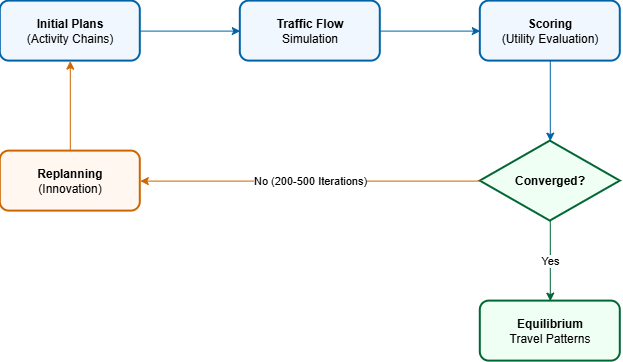Synthetic population distribution (adli, 2024). each data point represents a synthesised household and its associated agents, derived from census zone data via populationsim. 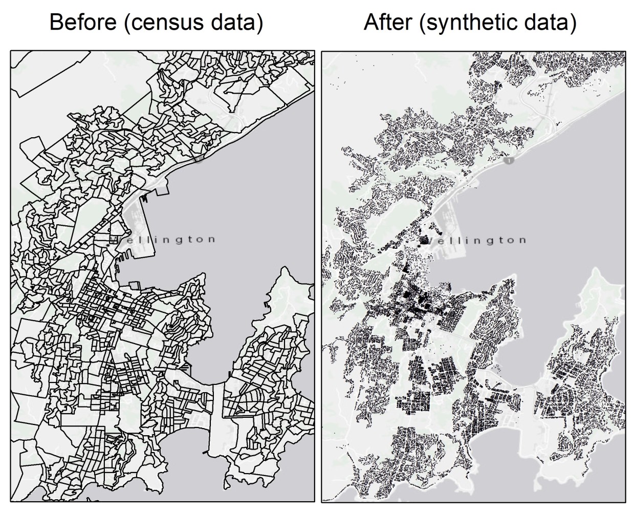Listing 1 provides a sample daily activity plan generated by ActivitySim, routing a synthetic agent based on census residence locations, household travel surveys (HTS), and origin-destination matrices (Adli, 2024).

Sample daily activity plan (activitysim XML output)

<person id="1195903">
  <attributes>
    <attribute name="household_id" class="java.lang.String">11959</attribute>
    <attribute name="age" class="java.lang.String">60</attribute>
    <attribute name="sex" class="java.lang.String">2</attribute>
    <attribute name="occupation" class="java.lang.String">Community and Personal Service Workers</attribute>
    <attribute name="home_sa1" class="java.lang.String">7001426</attribute>
    <attribute name="work_sa1" class="java.lang.String">7030907</attribute>
  </attributes>
  <plan selected="yes">
    <activity type="home" x="1750535.147" y="5950765.788" facility="osm:way:339490744:home" end_time="07:00:00"/>
    <leg mode="car" trav_time="00:28:04">
      <route type="generic" trav_time="00:28:04" distance="22737.0"/>
    </leg>
    <activity type="work" x="1755022.912" y="5931916.652" facility="osm:node:8340440533:work_service" end_time="17:00:00"/>
    <leg mode="car" trav_time="00:33:13">
      <route type="generic" trav_time="00:33:13" distance="19376.0"/>
    </leg>
    <activity type="home" x="1750535.147" y="5950765.788" facility="osm:way:339490744:home"/>
  </plan>
</person>

the annual land-use simulation (UrbanSim):

UrbanSim is a microsimulation platform for modelling urban development (Waddell, 2002; Waddell et al., 2003; Waddell, 2011). Its key characteristics are:

• Microsimulation: Individual households, firms, and real estate developers are the decision-making agents. Each agent has attributes (income, household size, industry, etc.) and makes location choices based on utility maximisation.

• Annual time steps: The model advances in one-year increments, with each year comprising a sequence of sub-model executions (demographic transitions, location choices, development, pricing).

• Spatial resolution: Decisions are modelled at the parcel or grid-cell level (150m × 150m), providing fine-grained spatial detail.

• Market clearing: Housing and commercial real estate markets clear through price adjustment. Excess demand raises prices, which dampens further demand.

Demographic transition model (DTM)

Before simulating spatial migration, the Demographic Transition Model accounts for the natural population dynamics of the urban system. Working on an annual cycle, the DTM applies age-specific fertility and mortality rates from ABS life tables to synthesise births and deaths, whilst aging all existing individuals by one year. The model also captures the lifecycle dynamics of household formation and dissolution, such as young adults leaving parental homes or households dissolving due to divorce or mortality. By constraining these micro-level transitions to align with ABS Series B population projections at the macroscopic level, the DTM ensures that the overall synthetic population grows at the correct aggregate trajectory. The subsequent location choice models are then responsible for determining precisely where this expanding population will spatially distribute.

Household location choice model (HLCM)

The HLCM determines where households choose to live. The utility of household i choosing dwelling h is: U_ih = β_a ⋅ A_h + β_c ⋅  cost_h + β_n ⋅  neighbourhood_h + ε_ih where A_h is the accessibility (logsum from MATSim), cost_h is the housing cost relative to income, neighbourhood_h captures attributes like school quality, and ε_ih is a Gumbel error term.

Key mechanism: When HSR improves accessibility A_h near stations, the utility of those locations increases, attracting households. This is the micro-level mechanism that generates macro-level population redistribution.

Employment location choice model (ELCM)

Firms select locations based on accessibility, land costs, and agglomeration benefits. The utility of firm f choosing location j is: U_jf = α₁ ⋅  Acc_j^labour  + α₂ ⋅  Acc_j^market  − α₃ ⋅  rent_j + α₄ ⋅  Agglom_j + ε_jf where Acc_j^labour and Acc_j^market are accessibilities computed from MATSim, rent_j is commercial rent, and Agglom_j is the density of complementary employment. SA4-level GDP informs the ELCM by constraining employment growth rates and industry composition.

Real estate price model (REPM)

The REPM determines property prices using a hedonic formulation: ln P_h = β₀ + β₁ ⋅  Acc_h + β₂ ⋅  size_h + β₃ ⋅  age_h + β₄ ⋅  neighbourhood_h + ε_h When HSR improves accessibility near stations, the REPM translates this into higher property prices, which feeds back into the HLCM (reducing affordability) and REDM (increasing development profitability).

Real estate development model (REDM)

Developers build where profitable, subject to zoning and land availability. The expected profit from developing parcel p is: Π_p =  Revenue_p −  Cost_p = (P_p ⋅ F_p) − (L_p + K_p ⋅ F_p) where P_p is expected sale price, F_p is developable floor area, L_p is land cost, and K_p is construction cost. The probability of development is a logistic function of expected profit, local vacancy, and zoning. This endogenises housing supply.

Why agent-based land use

The transition to an agent-based land use framework resolves several structural limitations inherent in traditional, aggregate models of spatial economics. Most fundamentally, the future population size of any given city or region is treated as an emergent output of the simulation rather than an exogenously imposed input. This growth manifests dynamically as heterogeneous households and firms—ranging from young professionals and families to manufacturing plants and corporate headquarters—exercise their distinct location preferences in response to changing transport accessibilities.

Moreover, this framework structurally grounds the urban housing market in microeconomic reality. Rather than relying on assumed, fixed elasticities for housing supply, the model allows supply constraints to emerge endogenously from the profit-maximising calculations of individual developers operating under strict local zoning and cost limitations. When an intervention such as HSR suddenly elevates the accessibility of a regional node, the ensuing surge in residential demand triggers the Real Estate Price Model to raise local property values. This price feedback acts as a vital market-clearing mechanism; the rising cost of land dampens unconstrained demand, preventing unrealistic population concentrations and ensuring the simulated spatial distribution remains economically viable.

Urbansim sub-models: key inputs, outputs, and data sources.

Urbansim annual cycle. the model executes demographic transitions, location choices, development, and price updates in sequence. accessibility feeds from MATSim into location choice and pricing.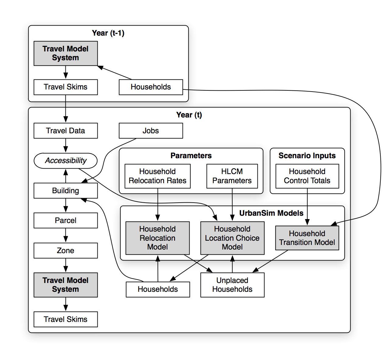

The three-loop coupling and convergence protocol

The coupling between SGE, MATSim, and UrbanSim operates through three nested feedback loops (illustrated in Figure 1):

1. Inner Loop (Daily Transport Market): MATSim runs to user equilibrium, updating link travel times and fares, and outputting zone-to-zone logsum accessibilities (A_i):

   A_i = ln ∑_j∑_mexp (V_ij, m)

2. Middle Loop (Annual Property Market): UrbanSim updates household and firm location distributions and real estate developer plans based on the latest accessibilities.

3. Outer Loop (Macro-Economic Market-Clearing): SGE market-clearing equations resolve wages w_j and floorspace rents q_i, adjusting the household’s endogenous value of travel time (υ_ij).

The entire system advances in annual steps until the logsum accessibility changes stabilise below the 1% threshold:

$$\max\limits_{i}\frac{~|~\left( A_{i}^{(k)} – A_{i}^{(k – 1)} \right)}{A_{i}^{(k – 1)}}~|~ < 0.01$$

Three-loop nested coupling protocol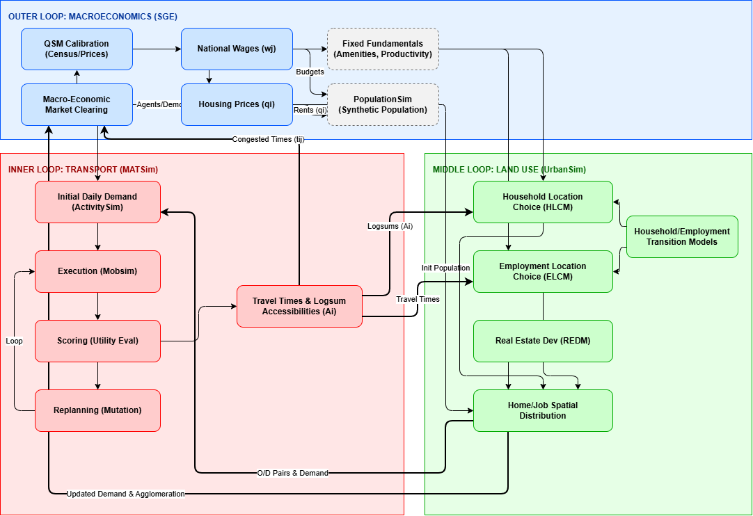

Conceptual case study: newcastle-to-melbourne corridor

The proposed East Coast High-Speed Rail network is a prime candidate for general equilibrium appraisal, as it represents a non-marginal infrastructure project that will structurally transform Australia’s eastern seaboard (Henn et al., 2012). The corridor spans over 1,000 kilometers and connects major metropolitan centres with intermediate regional cities.

Corridor geography and node categorisation

Our conceptual case study partitions the corridor into three distinct spatial hierarchies:

1. Metropolitan CBD Terminals: Sydney (Central) and Melbourne (Southern Cross) represent the primate economic engines of the corridor.

2. Primate Intermediate Terminals: Canberra and Newcastle represent major regional centres with diversified local economies.

3. Regional Commuter Terminals: Wollongong, Albury-Wodonga, Goulburn, and Seymour represent smaller, intermediate nodes.

   Corridor geography.

General equilibrium spatial scenarios

We simulate three spatial general equilibrium scenarios, which depend on the balance between agglomeration economies, housing supply elasticity (|(H)_i), and commuting tolerances:

Scenario A: metropolitan agglomeration dominance (Sydney and Melbourne)

Under this scenario, we assume high agglomeration elasticities (η) and highly restrictive regional zoning laws (low |(H)_i).

• Outcome: HSR dramatically strengthens business-to-business linkages and labour market pooling in Sydney and Melbourne CBDs, drawing high-skilled service firms and knowledge workers from intermediate regional hubs. The economic density and productivity of primate cities increase, but regional inequality widens as regional nodes suffer “straw-effect” drain (Bonnafous, 1987).

Scenario B: intermediate regional “function-borrowing” (Newcastle and Canberra)

Here, we assume moderate commuting tolerances and highly elastic housing and commercial floorspace supplies in intermediate regional hubs (high |(H)_i in Newcastle and Canberra).

• Outcome: Firms in the professional, scientific, and technical services sectors relocate from high-rent Sydney and Melbourne CBDs to Newcastle and Canberra. These intermediate regional hubs “borrow” the economic scale and labour markets of the primate cities via HSR, experiencing substantial wage and employment growth without suffering the cost of local metropolitan congestion (Ureña et al., 2009).

Scenario C: commuter-town residential capitalisation (Goulburn, Albury, Seymour)

This scenario assumes high household travel tolerance (willingness to utilise HSR for daily commutes of 45-60 minutes) and strict zoning limits in the primate CBDs.

• Outcome: High housing costs in Sydney and Melbourne push households to migrate to cheaper, high-amenity residential nodes along the corridor (e.g., Goulburn, Albury-Wodonga, and Seymour). These regional nodes capitalise accessibility gains into residential land values (rent uplift), transforming them into prosperous commuter dormitory towns with massive residential growth but limited local industrial development (Koster et al., 2024).

Contrasting with traditional LUTI system dynamics

The broader idea that transport interventions trigger delayed and interacting feedbacks across accessibility, economic activity, land use, and population dynamics has a long history within the LUTI literature. In particular, the system dynamics (SD) tradition, including the foundational work of Pfaffenbichler et al. (2010) on models such as MARS (Metropolitan Activity Relocation Simulator), has long employed causal-loop structures and feedback-based representations of transport–land use interactions operating over multiple temporal scales.

However, traditional SD models typically rely on aggregate stocks and flows governed by continuous differential equations and time delays. While computationally efficient for high-level strategy, they lack microeconomic foundations and treat households as fluid masses rather than utility-maximising individuals.

In contrast, our proposed LUTI model approach formalises this temporal causal chain through discrete microeconomic market-clearing. Instead of continuous time delays, temporal horizons are explicitly mapped to discrete nested simulation loops (the Daily MATSim transport loop, the Annual UrbanSim land-use loop, and the Annual SGE macroeconomic clearing loop). By clearing the market at the level of individual households and firms, the proposed framework provides high-resolution spatial and behavioural realism that aggregate SD approaches cannot achieve.

Welfare economics & SGE policy evaluation

To evaluate the overall economic return of the HSR corridor without the risk of double-counting or omitting secondary market spillovers, we adapt the spatial welfare decomposition of Donald et al. (2025) to our urban framework.

Sge welfare decomposition formulation

By applying the envelope theorem to the Lagrangian of the spatial general equilibrium pseudo-planning problem (see Appendix B for the full mathematical proof), the total welfare change (dW) induced by a transport intervention is decomposed into six additive, non-overlapping components:

$$\begin{aligned} dW & = \sum_{ij}\Lambda\mu_{ij} \cdot N_{ij}x_{ij} \cdot \left( – dt_{ij} \right) \\ & + N \cdot \operatorname{Cov}\left\lbrack \Lambda – \kappa_{ij}^{- 1},\kappa_{ij}p_{i} \cdot dC_{ij} \right\rbrack \\ & + N \cdot \operatorname{Cov}\left\lbrack \Lambda – \kappa_{ij}^{- 1},\kappa_{ij}q_{i} \cdot dH_{ij}^{R} \right\rbrack \\ & + \sum_{ij}\tau_{ij} \cdot d\left( N_{ij}x_{ij} \right) \\ & + \sum_{j}L_{j} \cdot dp_{\ell j} \\ & + \sum_{j}\frac{p\eta Y_{j}}{\rho_{j}} \cdot d\rho_{j} \end{aligned}$$

This decomposition represents:

1. Direct User Benefits (Term 1): The direct travel time savings (dt_ij) valued by the micro-founded marginal opportunity cost of time ($\frac{\mu_{ij}}{\kappa_{ij}}$).

2. Consumption Distribution Welfare (Term 2): The welfare effect of consumer re-sorting across the spatial income distribution, accounting for varying marginal utilities of income.

3. Housing Distribution Welfare (Term 3): The welfare impact of household reallocation across residential floorspace price gradients.

4. Operator Fare Revenues (Term 4): The direct financial impact on the rail operator through fare revenue changes (d(N_ijx_ij)).

5. Land Value Uplift (Term 5): The capitalisation of accessibility gains into land rents (dp_ℓj) captured by landowners.

6. Agglomeration Externality (Term 6): The endogenous shift in total factor productivity (Y_j) driven by changes in effective job accessibility (dρ_j).

Eliminating double-counting in appraisal

Because all six terms are derived from a single, unified Lagrangian system representing the general equilibrium state of the economy, the risk of double-counting is mathematically eliminated (Donald et al., 2025). For instance, standard PE appraisals often struggle to determine whether property price increases near HSR stations represent a new benefit or merely the capitalisation of travel time savings. In our SGE decomposition, the property value uplift (Term 5) is cleanly isolated from travel time savings (Term 1) and consumption reallocations (Term 2), providing a robust, theoretically consistent welfare metric for decision-makers.

Discussion and research agenda

The proposed LUTI model in this paper represents a significant advance in transport and land-use economics, yet several challenges and limitations remain to be addressed in future research.

Computational complexity and scalability

The integration of agent-based microsimulation models (MATSim and UrbanSim) with an SGE framework creates a computational bottleneck. Simulating individual agents over a 30-year planning horizon with iterative coupling requires high-performance computing (HPC) clusters and can take 24 to 48 hours for a single scenario run (Waddell et al., 2003). While sampling strategies (such as utilising a 10% representative sample of the synthetic population) mitigate the computational issue, they introduce statistical noise that can affect fine-grained, parcel-level real estate price predictions.

Integrating non-commuting travel purposes

A fundamental limitation of both current SGE models and traditional LUTI models is their restriction to commuting trips. Commuting journeys account for less than half of total transport consumption in modern metropolitan regions, a proportion that has further declined with the post-pandemic rise of remote work and telecommuting (Balbontin et al., 2024). High-Speed Rail networks are highly sensitive to non-commuting travel, as they draw substantial demand from business travel, tourism, and leisure. Integrating multi-purpose trip chains and non-commuting choices into an invertible SGE model represents a major theoretical challenge, as the mathematical properties of model inversion are typically proved only for simple, commuting-choice gravity formulations (Ahlfeldt et al., 2015). Recent advances in importance sampling and multidimensional choice modelling (Miyauchi et al., 2025) offer promising pathways to resolve this limitation.

Conclusions

Traditional transport appraisal frameworks are conceptually inadequate for evaluating transformative, capital-intensive infrastructure projects like High-Speed Rail. By focusing solely on direct transport user benefits in isolation, partial equilibrium models fail to capture the dynamic, feedback-driven reallocations of households and firms across space. While LUTI models address these reallocations, they lack a unified microeconomic welfare utility function, leading to double-counting and inconsistent appraisal metrics.

The proposed LUTI model appraoch presented in this paper resolves these issues by marrying the microeconomic welfare consistency of Spatial General Equilibrium with the high-resolution behavioural realism of agent-based microsimulation. By formalising a two-stage calibration-simulation protocol, we overcome the “invertibility-microsimulation” bottleneck, enabling the deterministic recovery of unobserved locational fundamentals and the dynamic simulation of agent-based choices under general equilibrium.

Conceptual application to Australia’s East Coast Newcastle-to-Melbourne HSR corridor demonstrates that the spatial general equilibrium outcomes, whether characterised by metropolitan dominance, regional function-borrowing, or commuter-town capitalisation, are highly sensitive to local housing supply elasticities and zoning constraints. By utilising a unified, non-overlapping general equilibrium welfare decomposition, our architecture provides policymakers with a mathematically rigorous, transparent, and welfare-consistent decision-making tool for evaluating nation-shaping transportation megaprojects.

Appendices

Appendix A: step-by-step derivation of household optimal choices

To derive the optimal choices of the household under separate monetary and temporal constraints, we maximise the Lagrangian function specified in [eq_lagrangian]:

Λ = U_ij − κ_ij[C_ij + q_iH_ij^R − x_ij(w_j − τ_ij)] − μ_ij[L_ij + x_ij(T + t_ij) − |(L)]

Taking the FOCs with respect to consumption C_ij and residential floorspace H_ij^R (from [eq_foc_c] and [eq_foc_h]):

$$\frac{\partial U_{ij}}{\partial C_{ij}} = \kappa_{ij}p_{i}\frac{\partial U_{ij}}{\partial H_{ij}^{R}} = \kappa_{ij}q_{i}$$

Dividing these two equations yields the marginal rate of substitution between consumption and housing, which must equal their price ratio:

$$\frac{\partial\frac{U_{ij}}{\partial}C_{ij}}{\partial\frac{U_{ij}}{\partial}H_{ij}^{R}} = \frac{p_{i}}{q_{i}}$$

Using the Cobb-Douglas subutility function K_ij = C_ij^β(H_ij^R)^1 − β, this reduces to:

$$\frac{\beta H_{ij}^{R}}{(1 – \beta)C_{ij}} = \frac{p_{i}}{q_{i}}q_{i}H_{ij}^{R} = \frac{1 – \beta}{\beta}p_{i}C_{ij}$$

Since the consumption good is the numeraire (p_i = 1), this implies that expenditures on housing are a fixed proportion of expenditures on tradable goods, governed by the housing budget share 1 − β:

C_ij = βY_ij^exp q_iH_ij^R = (1 − β)Y_ij^exp

where Y_ij^exp  = x_ij(w_j − τ_ij) is the total commuting net income.

Next, we evaluate the first-order condition with respect to leisure time L_ij ([eq_foc_l]):

$$\frac{\partial U_{ij}}{\partial L_{ij}} = \mu_{ij}$$

Isolating the Lagrange multipliers and substituting them into the labour supply FOC ([eq_foc_x]) yields:

$$C_{ij} = \frac{\gamma}{1 – \gamma}\beta\frac{\upsilon_{ij}L_{ij}}{p_{i}}$$

Substituting [eq_leisure_consumption_ratio] into the temporal budget constraint ([eq_temporal_budget]) and solving for leisure time L_ij yields the optimal leisure allocation:

L_ij = (1 − γ)|(L)

Substituting [eq_optimal_leisure] into [eq_leisure_consumption_ratio] yields the optimal consumption C_ij and residential floorspace H_ij^R specified in [eq_optimal_c] and [eq_optimal_h].

Appendix B: derivation of the SGE welfare decomposition

Following Donald et al. (2025) and Hörcher and Graham (2026), the decentralised equilibrium of our spatial economy solves a pseudo-planning problem whose Lagrangian is given by:

$$\begin{aligned} L & = W\left( E\left\lbrack U_{ij} \right\rbrack \right) + \sum_{ij}N\lambda_{ij}x_{ij}\tau_{ij} + \sum_{j}p_{\ell j}L_{j} \\ & + \widetilde{Y}\left\lbrack \sum_{j}A_{j}f_{y}\left( M_{j}^{W},H_{j}^{W} \right) – \sum_{ij}N\lambda_{ij}C_{ij} \right\rbrack \\ & + \sum_{j}{\widetilde{w}}_{j}\left\lbrack \sum_{i}N\lambda_{ij}x_{ij} – M_{j}^{W} \right\rbrack \\ & + \sum_{j}q_{j}\left\lbrack f_{h}\left( Z_{j},l_{j} \right) – \sum_{k}N\lambda_{jk}H_{jk}^{R} – H_{j}^{W} \right\rbrack \\ & + \sum_{j}{\widetilde{p}}_{\ell j}\left\lbrack L_{j} – l_{j} \right\rbrack \end{aligned}$$

We evaluate the total derivative of [eq_appendix_lagrangian] with respect to a transport policy intervention that induces small changes in the travel time matrix (dt_ij). By applying the envelope theorem, all derivatives of the Lagrangian with respect to the endogenous choice variables (λ_ij, C_ij, H_ij^R, x_ij, M_j^W, H_j^W, l_j) are identically zero at the equilibrium.

Therefore, the total change in welfare (dW) is given by the partial derivatives of the Lagrangian with respect to the exogenous travel time parameters:

$$dW = \frac{\partial L}{\partial t_{ij}}dt_{ij} + \frac{\partial L}{\partial A_{j}}\frac{\partial A_{j}}{\partial\rho_{j}}d\rho_{j}$$

Evaluating the partial derivative with respect to travel time (t_ij) yields:

$$\frac{\partial L}{\partial t_{ij}} = N\lambda_{ij}\left\lbrack \frac{\partial u_{ij}}{\partial L_{ij}}\frac{\partial L_{ij}}{\partial t_{ij}} \right\rbrack = – N\lambda_{ij}\mu_{ij}x_{ij}$$

Evaluating the partial derivative with respect to local productivities (A_j), accounting for the endogenous agglomeration elasticity (η), yields:

$$\frac{\partial L}{\partial A_{j}}dA_{j} = \frac{p\eta Y_{j}}{\rho_{j}}d\rho_{j}$$

Grouping the remaining terms for property values, operator fare revenues, and consumption reallocations yields the six-term additive welfare decomposition specified in [eq_welfare_decomp].

References

Acheampong, R. A., & Silva, E. A. (2015). Land use and transport interaction modelling: A review of the literature and future research directions. Journal of Transport and Land Use, 8(3), 11-38.

Ahlfeldt, G. M., Redding, S. J., Sturm, D. M., & Wolf, N. (2015). The economics of density: Evidence from the Berlin Wall. Econometrica, 83(6), 2127-2189.

Anas, A., & Liu, Y. (2007). A regional economy, land use, and transportation model (RELU-TRAN): Formulation, algorithm design, and testing. Journal of Regional Science, 47(3), 415-455.

Balbontin, C., Hensher, D. A., & Beck, M. J. (2024). The influence of working from home and underlying attitudes on the number of commuting and non-commuting trips by workers during 2020 and 2021 pre-and post-lockdown in Australia. Transportation Research Part A: Policy and Practice, 179, 103937.

Beria, P., Malkki, H., & Rodriguez-Nunez, E. (2012). Multi-criteria decision analysis in environmental and transport planning: A review. Science of the Total Environment, 409(19), 3578-3594.

Bonnafous, A. (1987). The regional impact of the TGV. Transportation, 14(2), 127-137.

Delventhal, M., & Parkhomenko, A. (2024). Spatial implications of telecommuting. Journal of Public Economics, 259, 105683.

Department for Transport. (2005). Transport Analysis Guidance: Introduction to Transport Analysis (TAG Unit 1.1). London: Department for Transport.

Doi, T. (2016). Interaction of Lifecycle Properties in High Speed Rail Systems Operation (Master’s thesis, Massachusetts Institute of Technology, Cambridge, MA).

Donald, E., Fukui, M., & Miyauchi, Y. (2025). Unpacking aggregate welfare in a spatial economy. NBER Working Paper Series, No. w34075.

Donaldson, D. (2018). Railroads of the raj: Estimating the impact of transportation infrastructure. American Economic Review, 108(4), 899-934.

Dupuit, J. (1844). De la mesure de l’utilité des travaux publics. Ouvres Économiques Complètes, 203-241.

Eliasson, J., & Fosgerau, M. (2019). Cost-benefit analysis of transport improvements in the presence of agglomeration and land-use externalities. Economics of Transportation, 19, 100121.

Graham, D. J., & Gibbons, S. (2019). Quantifying wider economic impacts of agglomeration for transport appraisal: Existing evidence and future directions. Economics of Transportation, 19, 100121.

Henn, L., Sloan, K., & Douglas, N. (2012). Towards a framework for evaluating financing alternatives for High Speed Rail along the East Coast of Australia. Australasian Transport Research Forum 2012 Proceedings, Perth.

Hörcher, D., & Graham, D. J. (2026). A quantitative urban model for transport appraisal. Journal of Public Economics, 259, 105683.

Horni, A., Nagel, K., & Axhausen, K. W. (Eds.). (2016). The Multi-Agent Transport Simulation MATSim. London: Ubiquity Press.

Hunt, J. D., & Simmonds, D. C. (1993). Theory and application of an integrated land-use and transport modelling framework. Environment and Planning B: Planning and Design, 20(2), 221-244.

Joint Transport Research Centre. (2008). The Wider Economic Benefits of Transport: Macro, Meso and Micro Transport Planning and Investment Tools (ITF Discussion Paper No. 2008-06). Paris: OECD/ITF.

Koster, H. R., Tabuchi, T., & Thisse, J. F. (2024). High-speed rail and the spatial distribution of economic activity: Evidence from Japan’s Shinkansen. RIETI Discussion Paper Series, No. 21-E-003.

Lowry, I. S. (1964). A Model of Metropolis (RM-4035-RC). Santa Monica, CA: RAND Corporation.

Marshall, A. (1920). Principles of Economics (8th ed.). London: Macmillan and Co.

Miyauchi, Y., Tsivanidis, N., & Redding, S. J. (2025). Evaluating the impact of urban transit infrastructure with multi-purpose trip chains. Journal of Urban Economics, 144, 103937.

Monte, F., Redding, S. J., & Rossi-Hansberg, E. (2018). Commuting, migration, and local employment elasticities. American Economic Review, 108(12), 3855-3890.

Pfaffenbichler, P., Emberger, G., & Shepherd, S. (2010). A system dynamics approach to land use transport interaction modelling: the strategic model MARS and its application. System Dynamics Review, 26(3), 262-282.

Proost, S., & Thisse, J. F. (2019). What can be learned from spatial economics? Journal of Economic Literature, 57(3), 575-643.

Redding, S. J., & Rossi-Hansberg, E. (2017). Quantitative spatial economics. Annual Review of Economics, 9, 21-58.

SACTRA. (1999). Transport and the Economy. London: The Stationery Office.

Tudela, A., Akiki, A., & Cisternas, R. (2006). Comparing CBA and MCA: An application to a Chilean transport project. Journal of Advanced Transportation, 40(3), 309-322.

Ureña, J. M., Menerault, P., & Garmendia, M. (2009). The high-speed rail challenge for big intermediate cities: A national, regional and local perspective. Cities, 26(5), 266-279.

Venables, A. J. (2007). Evaluating urban transport improvements: Cost-benefit analysis in the presence of agglomeration and income taxation. Journal of Transport Economics and Policy, 41(2), 173-188.

Waddell, P. (2002). UrbanSim: Modelling urban development for land use, transportation, and environmental planning. Journal of the American Planning Association, 68(3), 297-314.

Waddell, P., Borning, A., Noth, M., Freier, N., Becke, M., & Ulfarsson, G. (2003). Microsimulation of urban development and transportation: System architecture and results of an operational application of UrbanSim. Transportation Research Record, 1841, 71-80.

Wegener, M. (2004). Overview of land-use transport interaction models. Handbook of Transport Geography and Spatial Systems, 5, 127-146.

Wegener, M. (2011). Transport in spatial models of economic development. A Handbook on Transport Economics, 46-66.