Measuring accessibility
There is a subtle difference between transit accessibility and the accessibilities provided by other transportation modes. The main difference of transit accessibility is in its schedule. While travel time to/from transport and in-vehicle time is common between car and transit, the real test of freedom in transit relies on its spontaneity. Frequency has a direct role in the provision of freedom in transit and is the crucial variable in meeting the accessibility desires, yet, as Walker (2011) argues, the frequency is oddly invisible. Transit must exist in both space and time thus it must run not just where we need it but also when we need it. Unless it does both, it does not exist for us at all.
The cumulative-opportunity, or potential, approach and sums the number of essential destinations reachable within certain times by transit (Wachs and Kumagai, 1973; El-Geneidy and Levinson, 2006). This measure is particularly useful in describing how well transportation networks perform in relation to the distribution of destinations. This spontaneous nature of transit accessibility has made it more difficult to calculate the cumulative opportunity of a transit network. The Urban Access python library returns access/egress time, wait-time, number of transfers, or walking between transfers while providing the average wait time for transit services to factor in the spontaneity of a transit system.
Census data
Several sources of data on existing transport networks, population and employment locations were used. First, Open Street Map (OSM) has been used to model walking network geometry (e.g. street segments, stairs, restrictions and shortcuts). Second, General Transit Feed Specification (GTFS) data is used to model travel times and distances on transit networks. A GTFS feed comprises of a series of text files, where each file models one particular aspect of the system (for full description see Google, 2015). This study uses GTFS data valid for Thursday 12 October 2021. Third, population and employment data has been sourced from the Census 2018 data at the statistical area level 1.
Python code
import sys
import pathlib

import pandas as pd
import pandana as pdna
import geopandas as gpd

import urbanaccess as ua
from urbanaccess.config import settings
from urbanaccess.gtfsfeeds import feeds
from urbanaccess import gtfsfeeds
from urbanaccess.gtfs.gtfsfeeds_dataframe import gtfsfeeds_dfs
from urbanaccess.network import ua_network, load_network

DIR = pathlib.Path('..')
sys.path.append(str(DIR))

DATA_DIR = DIR/'data/'
GIS_DIR = DIR/'PT_Justice/'

nodes, edges = ua.osm.load.ua_network_from_bbox(
    bbox=(173.9053,-36.1068,175.3171,-37.3090),
)
ua.osm.network.create_osm_net(
    osm_edges=edges,
    osm_nodes=nodes,
    travel_speed_mph=3,
)

loaded_feeds = ua.gtfs.load.gtfsfeed_to_df(
    gtfsfeed_path=str((DATA_DIR/'Auckland_GTFS_20211014').resolve()),
)
ua.gtfs.network.create_transit_net(
    gtfsfeeds_dfs=loaded_feeds,
    day='thursday',
    timerange=['07:00:00', '09:00:00'],
)
ua.gtfs.headways.headways(
    gtfsfeeds_df=loaded_feeds,
    headway_timerange=['07:00:00','09:00:00'],
)

urbanaccess_net = ua.network.ua_network
ua.network.integrate_network(
    urbanaccess_network=urbanaccess_net,
    headways=True,
    urbanaccess_gtfsfeeds_df=loaded_feeds,
    headway_statistic='mean',
)

ua.network.save_network(
    urbanaccess_network=urbanaccess_net,
    filename='final_net.h5',
    dir=str(DATA_DIR.resolve()),
    overwrite_key = True,
)

transit_ped_net = pdna.Network(
    urbanaccess_net.net_nodes["x"],
    urbanaccess_net.net_nodes["y"],
    urbanaccess_net.net_edges["from_int"],
    urbanaccess_net.net_edges["to_int"],
    urbanaccess_net.net_edges[["weight"]],
    twoway=False,
)

census = gpd.read_file(
    GIS_DIR/'PT_Justice.gdb',
    driver='FileGDB',
    layer='census_2018_WGS84',
)
census['centroid'] = census.centroid
census['x'] = census.centroid.map(lambda x: x.x)
census['y'] = census.centroid.map(lambda y: y.y)

census['node_id'] = transit_ped_net.get_node_ids(census['x'], census['y'])

transit_ped_net.set(census.node_id, variable = census['Place_of_Work_2018'], name='jobs')
jobs_45 = transit_ped_net.aggregate(45, type='sum', decay='linear', name='jobs')

df = jobs_45.to_frame()
df.columns = ['jobs']
df['x']=transit_ped_net.nodes_df.x
df['y']=transit_ped_net.nodes_df.y
df.to_csv(DATA_DIR/'jobs_full.csv')
Results
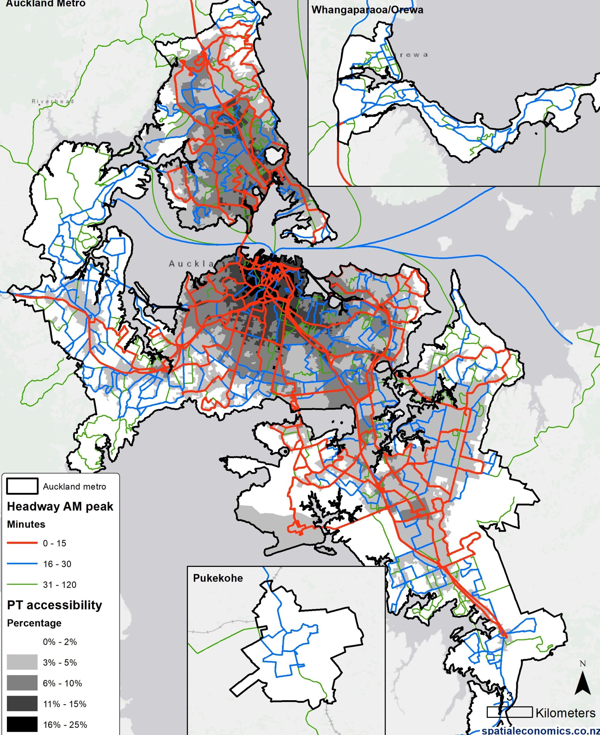
The accessibility analysis result shows the spatial distribution of PT accessibility in the Auckland region. The result is also available as a webmap.
References
El-Geneidy, A. and Levinson, D. M. (2006) Access to Destinations: Development of Accessibility Measures.
Google (2015) What is GTFS? Google. Available at: https://developers.google.com/transit/gtfs.
Walker, J. (2011) Human Transit: How Clearer Thinking about Public Transit Can Enrich Our Communities and Our Lives. Island Press.